|
|
RAY-TRACING
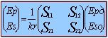
The LIDAR is, in most cases, vertically-pointing, and the only quantities that could be derived with different precision are the height-resolved volume backscatter [1(m sr)], the averaged volume extinction [1/m], and the degree of depolarization of the originally linearly-polarized laser light. The same information could be obtained at different wavelengths. All the microphysical information about the cloud should be retrieved from these (few and often noisy) LIDAR quantities…… |
The elastic-backscatter LIDAR is a powerful remote-sensing tool that produces vertical, 2-D, or 3-D qualitative maps of the distribution of aerosol backscatter in ice clouds. Even if LIDAR spatial and temporal resolutions are high enough to obtain an accurate maps of cloud backscatter, the precision and accuracy of the microphysical aerosol information that could be derived are affected by large uncertainties, even in the ideal case of a noiseless LIDAR.
|
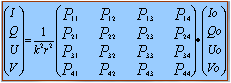
These LIDAR quantities are too few in order to retrieve the full optical properties of the particles!!! The basic elastic scattering process that takes place on cirrus particles illuminated with a plane wave can be described by the electrical field transformation matrix: |
Particles with very different orientations and shapes could in principle give similar Sij (Pij) elements, and they would thus be optically indistinguishable. If the scattering is measured at a single Q (Q =180° in the case of LIDAR), many more different ice particle shapes and orientations could give the same Sij(180°): this is why the microphysical interpretation of cirrus LIDAR data is so ambiguous…. If no special spatial orientations are expected for the ice particles, the scattering matrix can be averaged over all the possible 3-D orientations of the particle: in this case, the matrix loses its dependency on the particle orientation. In any case, it will still depend on particle shape, size, wavelenght and Q. By randomizing, some of the Pij elements vanish or show inter-relations due to reasons of symmetry. |
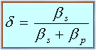
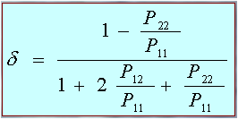
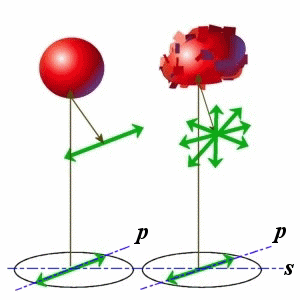
PARTICLE SYMMETRY is very important in LIDAR! When a linearly polarized laser beam (used in most LIDAR systems) hits a spherical particle, the 180° backscattered light must preserve its original polarization. This is a basic symmetry rule of Nature. When the shape is different, a depolarization of the backscattered light is expected. Several different definitions of LIDAR depolarization exist, in our case we use: |
 |
|
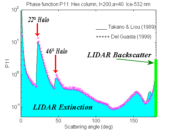
In the recent decades, powerful computers have made it possible to compute numerically the scattering properties of particles of a complex shape. Most simulations of cirrus optical properties have been carried out by means of ray-tracing techniques, in the hypothesis that ice particles larger than the wavelength dominated the size spectrum. Pristine hexagonal crystals (expected to be present in undisturbed cloud conditions) were extensively used in earlier simulations (Cai and Liou, 1982; Takano and Jayaweera, 1985; Takano and Liou, 1989; Muinonen et al., 1989; Hess and Wiegner, 1994; Zhang and Xu, 1995). The use of pristine hexagonal crystals in simulations make possible a correct prediction of the halos observed in some cirrus. An example of P11 for a pristine hex column oriented randomly in the space is reported here behind: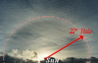 |
SIMULATION OF LIGHT SCATTERING BY LARGE NON-SPHERICAL PARTICLES WITH GEOMETRICAL OPTICS. |
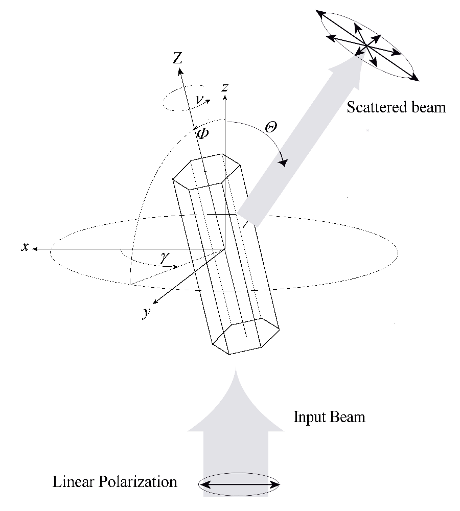
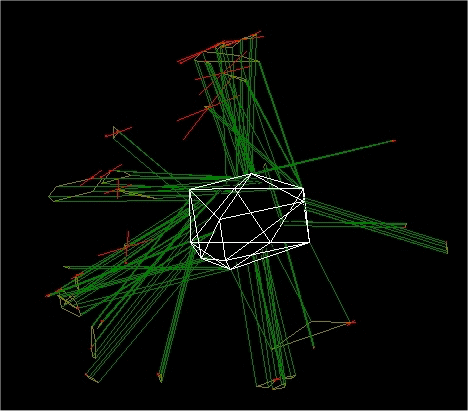
“Face-tracing” (FTR), is a numerical technique developed at IFAC CNR, is derived from ray-tracing. The technique permits the scattering to be simulated for convex, polyedral particles of an arbitrary shape. By using conventional ray-tracing techniques, single rays are traced into the particle, and the scattered energy is collected into solid angle intervals at different scattering angles so as to reconstruct the phase function. With the FTR technique, each face of the crystal illuminated by the LIDAR defines an initial finite beam which replaces the set of rays that illuminated the same face when the conventional technique was used. The projection of each face along the direction of the laser beam (z axis) defines the cross-section of the initial beam. The initial beam is reflected and refracted onto the “initial” face; the direction and the electric-field vector of the reflected and refracted beams are computed with the usual Snell and Fresnel laws. When proceeding within the particle, the refracted beam hits some faces of the solid internally, and is thus split into several sub-beams, one for each of the faces encountered. The intersection between the refracted beam and each encountered face is numerically computed, and the projection of this intersection along the refracted beam defines a new “sub-beam” which will later be reflected and refracted (or totally reflected) by the encountered face. The intersections between beams and faces are obtained numerically. The intersection between the beam and the face is a polygon, the vertices of which can be obtained numerically from the vertices of the projection and those of the face. This process is repeated for all the faces illuminated by the refracted beam, thus creating a sub-beam for each illuminated face. Each sub-beam created by the code undergoes the same process as the initial beam, by producing a reflected and a refracted beam. The beam-splitting process continues until a fixed amount (R’=99.5%) of the energy impinging on each illuminated face of the solid has been scattered in space. The process is repeated for all the illuminated faces of the crystal. An advantage of FTR is its ability to compute exactly the shape and the normal section of any scattered beam, which in turns makes it possible to compute the diffraction associated with each emerging beam. |
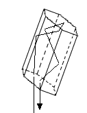
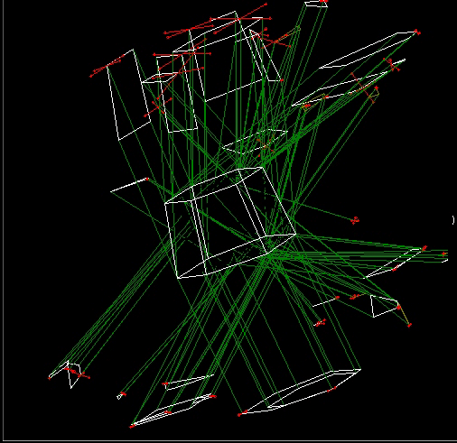
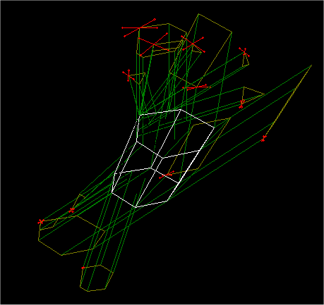
A snapshot of the “Face Tracing” process applied to a deformed Hex crystal. White polygons are the sections of the scattered beams. Red arrows show Ep,Es. |
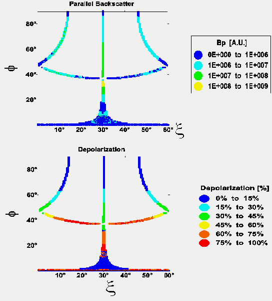
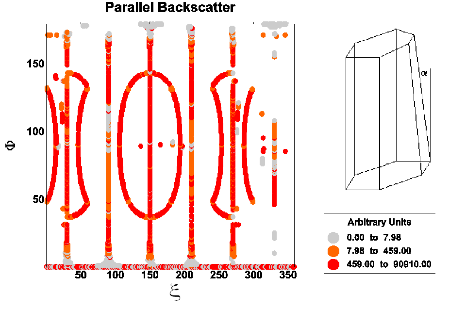
Many ray-paths lead to LIDAR backscatter in Hex crystals, but only a limited set of x and Q produce backscatter. The simplest paths, which involve a small number of internal reflections,usually lead to a low LIDAR depolarization. This occurs when the base or lateral faces of the crystal are almost horizontal (blue in dep. plot).With x and Q close to 30°, a special case occurs in which a complex ray-path leads to a depolarized corner-reflector effect (circled in purple). This effect is characteristic of ideal hex crystals, and disappears in deformed crystals. |
The origin of LIDAR backscatter in hexagonal crystals
|
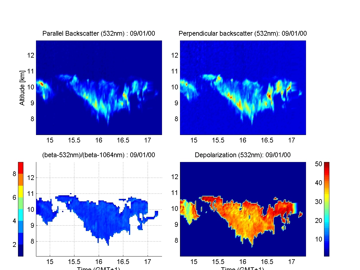
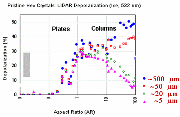
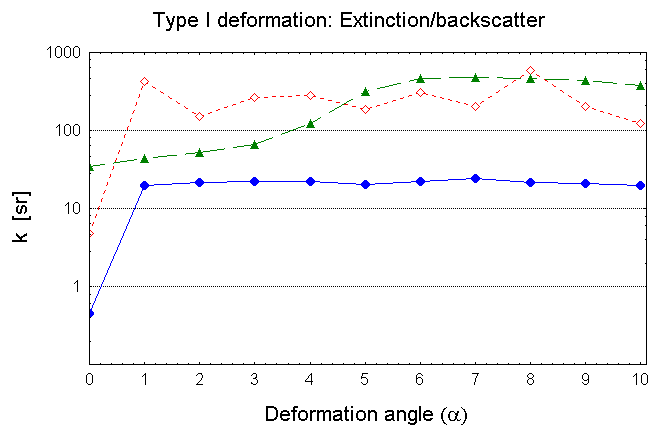
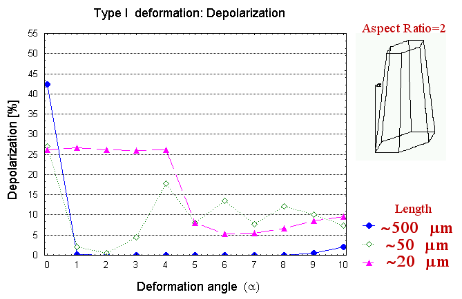
The Face Tracing results for the LIDAR quantities k and d are summarized if the figures below as functions of the crystal aspect ratio (length/diameter). Particles are randomly-oriented in space. Grey bars show the range of corresponding quantities as observed by LIDAR in Antarctic cirrus (midcloud T<-30°C, Del Guasta et al.,1993). Depolarization grows fast from almost 0 (very thin plates) up to 20-50% when the aspect ratio overcomes the unity. K values show a well-defined minimum for aspect ratio=1. In this case, the maximum backward transfer of energy occurs. K varies with the particle “diameter” because the backward scattering peak due to the corner reflector effect is smoothed out by diffraction in small particles. K values comparable with the observed ones are obtained by assuming relatively small ice crystals. |
|
The simple facts that halos are observed only seldom in nature, and that direct replicas of cirrus particles often show non-pristine crystals suggest that scattering simulations must be carried out on irregular particles. Ideal hexagonal particles also show a pronounced backscatter peak, which results in a very low extinction/backscatter ratio that is rarely observed in nature. The fact that optical properties of ice crystals often do not agree with simulations carried out with ideal ice particles has triggered the modeling of light scattering by more realistic, irregular ice particles. Particle aggregates such as bullet rosettes (Iaquinta et al., 1995), polyedral particles of different shapes (Takano and Liou, 1995; Macke, 1993), and deformed hexagonal crystals (Macke et al., 1996; Hess et al., 1998) have been modeled. In recent years, some fractal and irregular shapes have also been simulated using ray-tracing techniques (Macke et al., 1996; Mishchenko et al., 1996, Volten et al., 2001). Unfortunately, most ray-tracing simulations performed on ice crystals are not devoted to the LIDAR community, and the scattering quantities derived from these works (usually, the Pij elements) cannot be used easily by LIDAR teams. |
No Halos....................
|
Face Tracing can manage all sorts of polyedral particles, but computing time increases in the case of complicate geometries. Deformed hexagonal ice crystals were the first to be considered. Many different deformations that mantain the polyedral shape are possible . The x and F orientations of the crystal in space leading to backscatter become a complicated pattern even in the case of slight deformations. |
Face Tracing simulation for deformed Hexagonal ice crystals
|
LIDAR backscatter from deformed Hex crystals was found to be much weaker than that from pristine particles because the corner-reflector effect typical of the pristine crystals vanishes also for weak deformations. In the figures below, results of a bullet-like deformation are shown |
|
The simulation of scattering by irregular polyhedra is not new. Many researchers apply numerical techniques for this purpose, in order to simulate the scattering by realistic ice and dust particles. The face-tracing code has just started to work on these solids. Results will be available.....Acknowledgements This work was made possible under the Agenzia Spaziale Italiana contract ASI/CNR 1/R/073/01,“Simulazione numerica della diffusione della luce da parte dei cirri mediante tecnica di “ray-tracing” di seconda generazione. Applicazione delle simulazioni all’interpretazione delle misure LIDAR a depolarizzazione (532- 1064 nm) dallo spazio in termini di microfisica dei cirri” |
Face Tracing simulations for irregular polyedra
|
......Please download two papers about my Face-Tracing technique, in PDF !! |
|